pacman::p_load(tidyverse, tidymodels,
timetk, modeltime)20 Visualising, Analysing and Forecasting Time-series Data: timetk and modeltime methods
20.1 Learning Outcome
In this chapter, you will learn how to use timetk and model time packages to visualise, analyse and forescast time-series data. timetk provides a collection of functions for visualising and analysing time-series data. On the other hands, modeltime provides a collection of functions for time-series forecasting, both statistical learning and machine learning methods including deep learning and netsted forecasting methods.
In this topic, we are going to explore the tidymodels approach in time series forecasting.
- import and wrangling time-series data by using appropriate tidyverse methods,
- visualise and analyse time-series data,
- calibrate time-series forecasting models by using exponential smoothing and ARIMA techniques, and
- compare and evaluate the performance of forecasting models.
20.2 Setting Up R Environment
For the purpose of this hands-on exercise, the following R packages will be used.
tidyverse provides a collection of commonly used functions for importing, wrangling and visualising data. In this hands-on exercise the main packages used are readr, dplyr, tidyr and ggplot2.
modeltime a new time series forecasting package designed to speed up model evaluation, selection, and forecasting. modeltime does this by integrating the tidymodels machine learning ecosystem of packages into a streamlined workflow for tidyverse forecasting.
20.3 Introducing modeltime workflow
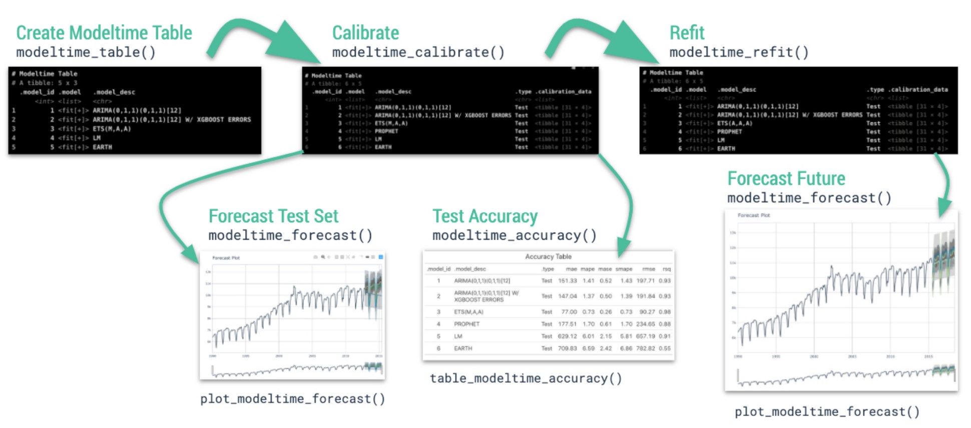
.small[ Source: Getting Started with Modeltime]
20.4 The data
In this sharing, Store Sales - Time Series Forecasting: Use machine learning to predict grocery sales from Kaggle competition will be used. For the purpose of this sharing, the main data set used is train.csv. It consists of six columns. They are:
- id contains unique id for each records.
- date gives the sales dates.
- store_nbr identifies the store at which the products are sold.
- family identifies the type of product sold.
- sales gives the total sales for a product family at a particular store at a given date. Fractional values are possible since products can be sold in fractional units (1.5 kg of cheese, for instance, as opposed to 1 bag of chips).
- onpromotion gives the total number of items in a product family that were being promoted at a store at a given date.
For the purpose of this sharing, I will focus of grocery sales instead of all products. Code chunk below is used to extract grocery sales from train.csv and saved the output into an rds file format for subsequent used.
store_sales <- read_csv(
  "data/store_sales/train.csv") %>%
  filter(family == "GROCERY I") %>%
  write_rds("data/store_sales/grocery.rds")
20.5 Time Series Forecasting Process
- Collect data and split into training and test sets
- Create & Fit Multiple Models
- Add fitted models to a Model Table
- Calibrate the models to a testing set.
- Perform Testing Set Forecast & Accuracy Evaluation
- Refit the models to Full Dataset & Forecast Forward
20.5.1 Step 1: Data Import and Sampling
In the code chunk below, read_rds() of readr package is used to import both data sets into R environment.
grocery <- read_rds(
  "data/store_sales/grocery.rds") %>%
  mutate(across(c(1, 3, 4),
                as.factor)) %>%
  group_by(family, date) %>%
  summarise(sum_sales = sum(sales)) %>%
  ungroup()
Optionally, you can also import the rest of the data sets provided at Kaggle by using the code chunk below.
holidays_events <- read_csv(
  "data/store_sales/holidays_events.csv")
oil <- read_csv(
  "data/store_sales/oil.csv")
stores <- read_csv(
  "data/store_sales/stores.csv")
transactions <- read_csv(
  "data/store_sales/transactions.csv")
20.5.2 Step 1: Data Import and Sampling
grocery tibble data frame consists of 1684 days of daily sales data starts from 1st January 2013. We will split the data set into training and hold-out data sets by using initial_time_split() of rsample package, a member of the tidymodels family.
splits <- grocery %>%
  initial_time_split(prop = 0.955)
For checking purposes, the code chunk below can be used save the split sample data sets into training and holdout tibble data tables respectively.
training <- training(splits)
holdout <- testing(splits)
20.5.3 Step 2: Create & Fit Multiple Models
In this step, we will build and fit four models using the code chunks below:
Model 1: Exponential Smoothing (Modeltime)
An Error-Trend-Season (ETS) model by using exp_smoothing().
model_fit_ets <- exp_smoothing() %>%
    set_engine(engine = "ets") %>%
    fit(sum_sales ~ `date`,
        data = training(splits))
Model 2: Auto ARIMA (Modeltime)
An auto ARIMA model by using arima_reg().
model_fit_arima <- arima_reg() %>%
  set_engine(engine = "auto_arima") %>%
  fit(sum_sales ~ `date`,
      data = training(splits))
Model 3: Boosted Auto ARIMA (Modeltime)
An Boosted auto ARIMA model by using arima_boost().
model_fit_arima_boosted <- arima_boost(
  min_n = 2,
  learn_rate = 0.015) %>%
  set_engine(
    engine = "auto_arima_xgboost") %>%
  fit(sum_sales ~ `date`,
      data = training(splits))
Model 4: prophet (Modeltime)
A prophet model using prophet_reg().
model_fit_prophet <- prophet_reg() %>%
  set_engine(engine = "prophet") %>%
  fit(sum_sales ~ `date`,
      data = training(splits))
20.5.4 Step 3: Add fitted models to a Model Table
Next, modeltime_table() of modeltime package is used to add each of the models to a Modeltime Table.
models_tbl <- modeltime_table(
  model_fit_ets,
  model_fit_arima,
  model_fit_arima_boosted,
  model_fit_prophet)

models_tbl
# Modeltime Table
# A tibble: 4 × 3
.model_id .model .model_desc
<int> <list> <chr>
1 1 <fit[+]> ETS(M,N,M)
2 2 <fit[+]> ARIMA(3,0,0)(1,1,2)[7]
3 3 <fit[+]> ARIMA(1,0,3)(2,1,2)[7]
4 4 <fit[+]> PROPHET 20.5.5 Step 4 - Calibrate the model to a testing set
In the code chunk below, modeltime_caibrate() is used to add a new column called .calibrate_data into the newly created models_tbl tibble data table.
calibration_tbl <- models_tbl %>%
    modeltime_calibrate(new_data = testing(splits))

calibration_tbl
# Modeltime Table
# A tibble: 4 × 5
.model_id .model .model_desc .type .calibration_data
<int> <list> <chr> <chr> <list>
1 1 <fit[+]> ETS(M,N,M) Test <tibble [76 × 4]>
2 2 <fit[+]> ARIMA(3,0,0)(1,1,2)[7] Test <tibble [76 × 4]>
3 3 <fit[+]> ARIMA(1,0,3)(2,1,2)[7] Test <tibble [76 × 4]>
4 4 <fit[+]> PROPHET Test <tibble [76 × 4]>Note that Calibration Data is simply forecasting predictions and residuals that are calculated from the hold-out data (also know as test data in machine learning)
20.5.6 Step 5: Model Accuracy Assessment
In general, there are two ways to assess accuracy of the models. They are by means of accuracy metrics or visualisation.
In the code chunk below, modeltime_accuracy() of modeltime package is used compute the accuracy metrics. Then, table_modeltime_accuracy() is used to present the accuracy metrics in tabular form.
calibration_tbl %>%
  modeltime_accuracy %>%
  table_modeltime_accuracy(
.interactive = FALSE)| Accuracy Table | ||||||||
|---|---|---|---|---|---|---|---|---|
| .model_id | .model_desc | .type | mae | mape | mase | smape | rmse | rsq |
| 1 | ETS(M,N,M) | Test | 25250.52 | 9.86 | 0.65 | 9.61 | 31554.80 | 0.64 |
| 2 | ARIMA(3,0,0)(1,1,2)[7] | Test | 23087.67 | 8.90 | 0.59 | 8.79 | 29863.72 | 0.66 |
| 3 | ARIMA(1,0,3)(2,1,2)[7] | Test | 23049.21 | 8.89 | 0.59 | 8.78 | 29829.18 | 0.66 |
| 4 | PROPHET | Test | 22356.01 | 8.54 | 0.57 | 8.60 | 30521.52 | 0.66 |
Visualizing the Test Error is easy to do using the interactive plotly visualization (just toggle the visibility of the models using the Legend).
calibration_tbl %>%
  modeltime_forecast(
    new_data = testing(splits),
    actual_data = grocery) %>%
  plot_modeltime_forecast(
    .legend_max_width = 25,
    .interactive = TRUE,
    .plotly_slider = TRUE)
20.5.7 Step 6 - Refit to Full Dataset & Forecast Forward
The final step is to refit the models to the full dataset using modeltime_refit() and forecast them forward.
The code chunk below uses modeltime_refit() to refit the forecasting models with the full data.
refit_tbl <- calibration_tbl %>%
    modeltime_refit(data = grocery)
Then, modeltime_forecast() is used to forecast to a selected future time period, in this example 6 weeks.
forecast_tbl <- refit_tbl %>%
  modeltime_forecast(
    h = "6 weeks",
    actual_data = grocery,
    keep_data = TRUE)
Notice that this newly derived forecast_tbl consists of 1852 rows (1684 rows for the original grocery sales data plus 7 days x 6 weeks x 4 models forecasted data)
forecast_tbl %>%
  plot_modeltime_forecast(
    .legend_max_width = 25,
    .interactive = TRUE,
    .plotly_slider = TRUE)
Let us also examine the model accuracy metrics after refitting the full data set.
refit_tbl %>%
  modeltime_accuracy() %>%
  table_modeltime_accuracy(
.interactive = FALSE)| Accuracy Table | ||||||||
|---|---|---|---|---|---|---|---|---|
| .model_id | .model_desc | .type | mae | mape | mase | smape | rmse | rsq |
| 1 | ETS(M,N,M) | Test | 25250.52 | 9.86 | 0.65 | 9.61 | 31554.80 | 0.64 |
| 2 | ARIMA(3,0,0)(1,1,2)[7] | Test | 23087.67 | 8.90 | 0.59 | 8.79 | 29863.72 | 0.66 |
| 3 | UPDATE: ARIMA(4,0,4)(1,1,2)[7] WITH DRIFT | Test | 23049.21 | 8.89 | 0.59 | 8.78 | 29829.18 | 0.66 |
| 4 | PROPHET | Test | 22356.01 | 8.54 | 0.57 | 8.60 | 30521.52 | 0.66 |